GIS 4930 - Project 4 - Analyze - Food Deserts

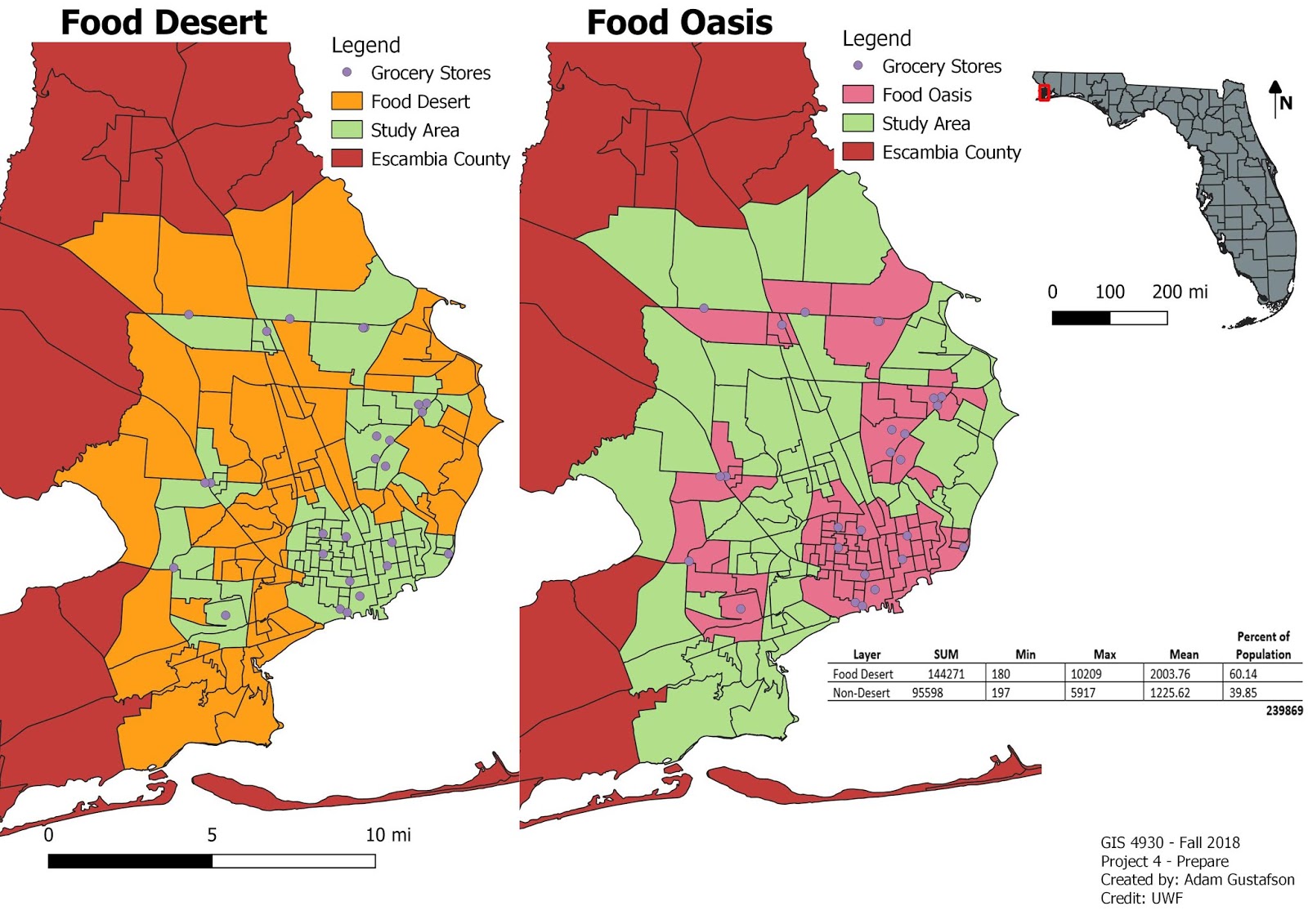
For this weeks portion of Project 4 we were tasked with taking the food desert and grocery store shape file data we created last week and uploading them into two open source web map making programs, Mapbox and Leaflet.
Using mapbox I was able to design a layout with a graduated symbology split into five classes based on  fooddesert.shp's pop2000 field.

Using the quickstart guide, and the project procedures I was able to create a marker displaying 2 text lines, a circle in a food oasis area, and a 4 coordinate polygon in a food desert area.

Some problems that I ran into over the course of this weeks project include: not being able to locate the correct mapbox to leaflet link required to transfer the maps tileset. Therefore my fooddeserts and grocerystores files are not displayed on my leaflet map.

Link to mapbox map displaying tileset

GIS 4930 - Project 4 - Prepare - Food Deserts

"food desert"     
an urban area in which it is difficult to buy affordable or good-quality fresh food.
-dictionary.com

For this weeks portion of project 4 we were tasked with preparing two maps, using Qgis , showing areas in Escambia county that would be considered food areas or food deserts. Areas were subjected to a proximity selection based on nearness to grocery stores. The following deliverables were created in qgis: a map showing Escambia county and UWFs location and a map showing food deserts and food oasis with the project 4 study area as background. The following population statistics were calculated : food desert 60.14% of total pop, food oasis 39.85% of total pop.

GIS 4035 - Module 10 - Germantown, MD - Supervised Classification

This week we were tasked with another image classification project. For this project a 57.42 square mile study area located in Germantown, Maryland was subjected to a supervised classification. The following classification consisted of a recording to 8 categories. The 8 categories are as follows: Urban, Grass, Deciduous Forest, Mixed Forest, Fallow Field, Agriculture, Water, and Road. The following features were selected for visually and based on provided coordinates using a drawn polygon method and the region growing properties > at inquire > spectral euclidean value method. The spectral euclidean value and the neighborhood value were adjusted accordingly to obtain features in which there was minimal spectral overlap.
The attached map deliverable highlights the 8 feature categories and their corresponding areas in square miles. The Spectral Euclidean distance map shows a representation of spectral Euclidean distance with brighter areas being represented as values with a larger pixel difference thus having a higher likelihood for wrong classification. The inset spectral Euclidean Distance map is overall dark indicating correct classification.

GIS 4035 - Module 9 - Unsupervised Classification

This week we were tasked with performing an unsupervised classification of our very own UWF campus here in Pensacola, Florida. The unsupervised classification was ran using ERDAS.
UWFclass50.img was created with the following settings : classes 50, RGB 321, maximum iterations 25,
convergence threshold 0.950, skip factors x: 2 y: 2.  Attribute table data was opened and the following category names were applied to the following pixel features in the UWFclass50.img:
Trees – dark green, Grass – green or chartreuse, Buildings/Road – grey,
Shadows – black, Mixed – light green
All 50 classes were recolored and renamed T, G, B, S, or M
Area was manually calculated and determined to be .90 square miles. Impervious percentage
calculated as 25% and Pervious percentage calculated as 75%.

GIS 4930 - Project 3: Analysis - Statistical Analysis of Methamphetamine Laboratory Busts

For this week's portion of Project 3 we were tasked with running an Ordinary Least Square regression on our data compiled in the previous week.

An ordinary least square regression method involves comparing a dependent variable (meth lab density) and explanatory (independent) variables. The explanatory variables consist of census data and the following variables were chosen: Males, Females, Age_18_21, Age_22_29, Age_30_39, Age_40_49, Age_50_64, Age_65_ Up, Hsehld_1_M, Hsehld_1_F, HSE_Units, and Vacant. The following variables were chosen based on review of the following three resulting values: Probability, Coefficient, and VIF. Values with probability > 1.0 were immediately removed as these values indicate low statistical significance. Variable coefficient values were taken into account as they indicate the relationship between the dependent variable and the explanatory variables indicating a strong or weak relationship. VIF values indicate overrepresentation or overlapping data amongst similar explanatory variables. Variables Males, Females, and HSE_Units all had a high VIF value as they were overrepresented in the census data. This does not necessarily denote a negative aspect seeing as how all participants had to choose one of two choices, Male or Female. This overrepresentation indicated from high VIF values is to be expected.

Attached is my results for OSL results displayed as STDResidual on the study area map and my OSL results in table form