INTRO GIS4043 - Lab 7-8 Data Search Midterm

"Success is the result of perfection, hard work, learning from failure, loyalty, and persistence." -Colin Powell

Over the last two weeks we were assigned a Florida county and tasked with creating a set of maps that would display the following data: roads, rivers, county boundaries, city names, public lands, digital elevation model image, digital orthophoto quarter quadrangle image, and two environmental categories. The county that I was assigned was Manatee County. I chose wetlands and invasive species for the two environmental shapefiles. 
After compiling all of the data from multiple databases including: Labins.org, FGDL.org, and nationalmap.gov, I came to the conclusion that three maps would be the best for displaying all of this data.
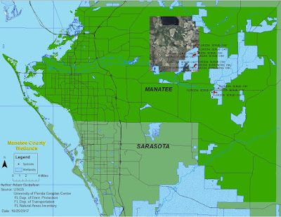
My first map consists of wetlands locations and species that occupy these areas. I constructed this map from a single data frame and transformed all shapefiles to the single projection of

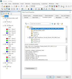
NAD_1983_2011_StatePlane_Florida_West_FIPS_0902_Ft_US. On this map I included shapefiles for rivers, roads, county boundaries, wetlands,and species. A DOQQ consisting of 4 quadrants (2919) was also added to this map in order to show some terrain features of one of the larger wetlands areas.
My second map consists of state park locations within the boundaries of Manatee County. This map was constructed with two data frames so a shapefile of the state of florida could be displayed with the location of Manatee County highlighted to show location. All shapefiles on the stateparks map were transformed in order to maintain a single projection. City names and state parks were labeled and displayed via a legend in order to display information effectively.   
My third map consists of a digital elevation model clipped to the boundaries of Manatee County.
This final step in the project proved to be the most challenging. In order to obtain a proper clip I had to export a shapefile of Manatee County separating it from the County Boundary file of the entirety of Florida. Once this was achieved I was able to use the Clip (data managment) tool to clip the raster file to conform to the shape of Manatee County perfectly. A suitable elevation gradient color was chosen to reflect low areas as greenish shades and higher areas as reddish shades.
Overall this project was dense but as is to be expected for a two week midterm. I am pleased with the outcome.

Success is the result of perfection, hard work, learning from failure, loyalty, and persistence. Colin Powell
Read more at: https://www.brainyquote.com/quotes/keywords/persistence.html

Success is the result of perfection, hard work, learning from failure, loyalty, and persistence. Colin Powell
Read more at: https://www.brainyquote.com/quotes/keywords/persistence.html

INTRO GIS4043 - Lab 6 Projections Continued

Understanding that every projection distorts is the key to figuring out which projection you need to use.

In this weeks lab we were tasked with creating multiple shapefiles from a multitude of sources and assembling all of this information into a single .mxd in Arcmaps with a uniform projection. To begin we were introduced to two data storage sites, Labins.org and FGDL.org. These websites specialize in storage and download of Florida mapping files, including but not limited to aerial photography, wildlife distribution, roads, rivers, and a multitude of other files.
For my final submission I used Labins.org to pull four aerial photography files in raster form (.sid) for quadrant 5159 in Escambia county Florida. These four quadrant files (NE,NW,SE, and SW) were projected as NAD_1983_StatePlane_Florida_North_FIPS_0903_Feet and applied as four seperate layers.
The second layer of my final submission required the use of FGDL.org in order to download a shapefile of Floridas major roads. This data file came projected in Albers Conical Equal Area but through the use of the project(data management) tool the file was reprojected to NAD_1983_2011_StatePlane_Florida_North_FIPS_0903_Ft_US. 

The third layer consisted of county boundaries with the above mention state plane projection. 

The fourth layer consisted of stateplane quadrants reprojected in the above mentioned state plane projection.

The fifth and final layer involved conversion of an excel data sheet of petroleum storage tank contamination monitoring sites in Escambia County into a shapefile and imported over the existing layers. For this data sheet to align correctly the given coordinates (in DMS) were converted into decimal degrees and imported into Arcmaps with the WGS_1984 projection then reprojected into the above mentioned state plane projection.

The final result (pictured below) resulted from the understanding of projections, the project(data managment) reprojection tool, and accessing data files in the above mentioned data storage websites.