GIS 4930 - Project 4 - Analyze - Food Deserts

For this weeks portion of Project 4 we were tasked with taking the food desert and grocery store shape file data we created last week and uploading them into two open source web map making programs, Mapbox and Leaflet.
Using mapbox I was able to design a layout with a graduated symbology split into five classes based on  fooddesert.shp's pop2000 field.

Using the quickstart guide, and the project procedures I was able to create a marker displaying 2 text lines, a circle in a food oasis area, and a 4 coordinate polygon in a food desert area.

Some problems that I ran into over the course of this weeks project include: not being able to locate the correct mapbox to leaflet link required to transfer the maps tileset. Therefore my fooddeserts and grocerystores files are not displayed on my leaflet map.

Link to mapbox map displaying tileset

GIS 4930 - Project 4 - Prepare - Food Deserts

"food desert"     
an urban area in which it is difficult to buy affordable or good-quality fresh food.
-dictionary.com

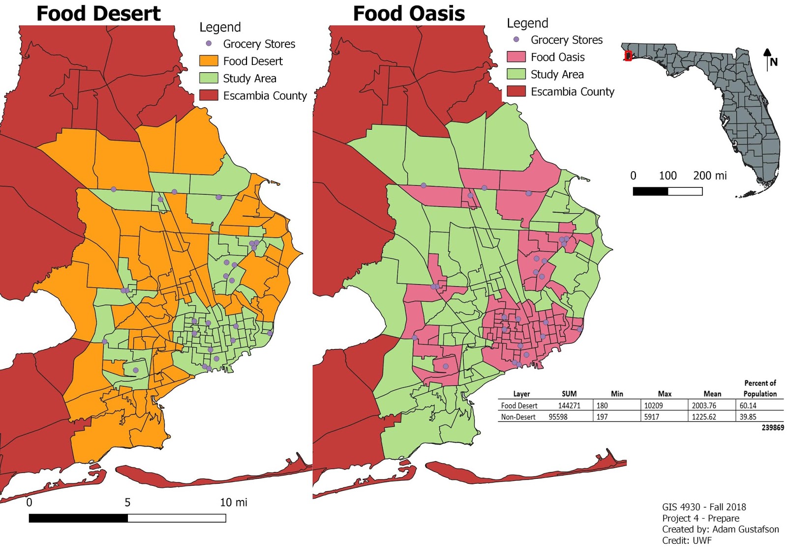
For this weeks portion of project 4 we were tasked with preparing two maps, using Qgis , showing areas in Escambia county that would be considered food areas or food deserts. Areas were subjected to a proximity selection based on nearness to grocery stores. The following deliverables were created in qgis: a map showing Escambia county and UWFs location and a map showing food deserts and food oasis with the project 4 study area as background. The following population statistics were calculated : food desert 60.14% of total pop, food oasis 39.85% of total pop.

GIS 4035 - Module 10 - Germantown, MD - Supervised Classification

This week we were tasked with another image classification project. For this project a 57.42 square mile study area located in Germantown, Maryland was subjected to a supervised classification. The following classification consisted of a recording to 8 categories. The 8 categories are as follows: Urban, Grass, Deciduous Forest, Mixed Forest, Fallow Field, Agriculture, Water, and Road. The following features were selected for visually and based on provided coordinates using a drawn polygon method and the region growing properties > at inquire > spectral euclidean value method. The spectral euclidean value and the neighborhood value were adjusted accordingly to obtain features in which there was minimal spectral overlap.
The attached map deliverable highlights the 8 feature categories and their corresponding areas in square miles. The Spectral Euclidean distance map shows a representation of spectral Euclidean distance with brighter areas being represented as values with a larger pixel difference thus having a higher likelihood for wrong classification. The inset spectral Euclidean Distance map is overall dark indicating correct classification.

GIS 4035 - Module 9 - Unsupervised Classification

This week we were tasked with performing an unsupervised classification of our very own UWF campus here in Pensacola, Florida. The unsupervised classification was ran using ERDAS.
UWFclass50.img was created with the following settings : classes 50, RGB 321, maximum iterations 25,
convergence threshold 0.950, skip factors x: 2 y: 2.  Attribute table data was opened and the following category names were applied to the following pixel features in the UWFclass50.img:
Trees – dark green, Grass – green or chartreuse, Buildings/Road – grey,
Shadows – black, Mixed – light green
All 50 classes were recolored and renamed T, G, B, S, or M
Area was manually calculated and determined to be .90 square miles. Impervious percentage
calculated as 25% and Pervious percentage calculated as 75%.

GIS 4930 - Project 3: Analysis - Statistical Analysis of Methamphetamine Laboratory Busts

For this week's portion of Project 3 we were tasked with running an Ordinary Least Square regression on our data compiled in the previous week.

An ordinary least square regression method involves comparing a dependent variable (meth lab density) and explanatory (independent) variables. The explanatory variables consist of census data and the following variables were chosen: Males, Females, Age_18_21, Age_22_29, Age_30_39, Age_40_49, Age_50_64, Age_65_ Up, Hsehld_1_M, Hsehld_1_F, HSE_Units, and Vacant. The following variables were chosen based on review of the following three resulting values: Probability, Coefficient, and VIF. Values with probability > 1.0 were immediately removed as these values indicate low statistical significance. Variable coefficient values were taken into account as they indicate the relationship between the dependent variable and the explanatory variables indicating a strong or weak relationship. VIF values indicate overrepresentation or overlapping data amongst similar explanatory variables. Variables Males, Females, and HSE_Units all had a high VIF value as they were overrepresented in the census data. This does not necessarily denote a negative aspect seeing as how all participants had to choose one of two choices, Male or Female. This overrepresentation indicated from high VIF values is to be expected.

Attached is my results for OSL results displayed as STDResidual on the study area map and my OSL results in table form

GIS 4035 - Module 8 - Thermal and Multispectral Imagery

For this week's Module 8 we were asked to analyze two composite satellite images at different RGB and landsat band setups in order to highlight specific features. The composite image that I chose was the EMTcomposite.img created in module 8 and the feature I chose to identify was the two fires located in the NE corner of the original EMTcomposite.img. I chose 4 data frames to show 4 different image configurations. These 4 data frames represent, in my opinion, the most effective ways to spot a forest fire via satellite imagery. The configuration of the 4 data frames is as following: RGB 123 - True color image for comparison, RGB 137 – fire appears brighter and more vivid, Landsat Band 1 – Grey Scale – shows brighter areas, Landsat Band 1 – Color Gradient – shows brighter areas as red. Landsat band 1 was chosen as it is the only band that effects the fire. This may be in part due to the fires intense brightness and its physical appearance being higher in elevation when compared to surrounding ground elevation.

GIS 4035 - Module 7 - Multispectral Analysis

This week, for module 7, we were tasked with analyzing satellite imagery for a mountain range in Washington state, tm_00.img. By analyzing histogram data one can extrapolate important information about the .img file.
The following map deliverable focuses on three features located in the tm_00.img.
Feature 1 criteria: In Layer_4 there is a spike between pixel values of 12 and 18. Name the type of feature responsible for this and locate an example of it on the map.
Feature 2 criteria: Identify the feature that represents both A) a small spike in layers 1-4 around pixel value 200, and B) a large spike between pixel values 9 and 11 in Layer_5 and Layer_6.
Feature 3 criteria:  In certain areas of water, layers 1-3 to become much brighter than normal, 
layer 4 becomes somewhat brighter, and layers 5-6 to remain unchanged. Locate an example area that clearly shows these variations in water, using a band combination that makes them stand out.

The following map deliverable was created in arcMap highlighting all 3 features and showing their location in the original tm_00.img with colored extent indicators. The following RGB band combinations are listed as legends for each corresponding feature and an explanation for how I located the feature is found to the right of each corresponding feature.

GIS 4930 - Project 3: Prepare - Statistical Analysis of Methamphetamine Laboratory Busts

"Most illicit drugs present two serious problems for society. First are the many consequences of drug use for the user, the community, and society as a whole. Second is the violence that accompanies the business of drugs that are transported across national borders through elaborate networks. Methamphetamine contributes to both problems, but in many parts of the country it presents another serious problem, namely the social and environmental damage that comes from domestic methamphetamine production." Methamphetamine Laboratories: The Geography of Drug Production - Ralph A. Weisheit and L. Edward Wells

For this week’s portion of Project 3: Prepare, we were tasked with preparing for a Statistical Analysis of Methamphetamine Laboratory Busts in West Virginia, USA. The final report for this module will consist of a fully constructed multi paged scientific analysis of the West Virginia study area comparing specific census tract demographics to the location of reported meth lab clusters. This analysis will serve to solidify any doubt in regards to medical, property and economical damage, that this drug and the drugs creation processes has wrought on West Virginia over the last few decades. I look forward to performing this analysis and to next week’s ordinary least square regression model creation.

Below is a constructed basemap of the study area with all essential map elements for the module 3 project.

GIS 4035 - Module 6 - Spatial Enhancement

"The Landsat 7 sensor suffered a malfunction in 2003 called a Scan Line Corrector failure. Since then, Landsat 7 images have frequent lines of no data, giving the images a striped appearance." -Module 6 Background

For this weeks module we were tasked with enhancing a .img file of satellite imagery using Erdas Imagine. Utilizing Erdas one can edit an image in an assortment of ways and this module goes into depth into a variety of filters and tools that can be utilized in order to enhance an area to highlight certain features or in the case of l7_striping.img fix large gaps running diagonally through the image caused by satellite processing malfunction. The main tools used in order to correct for this malfunction were the Fourier Transform, Fourier Transform Editor, Spatial Convolution, and Focal Statistics. A preview of the Fourier Editor settings is included in the attached map and shows the technique I used in order to hide the gaps by applying wedge voids to the "star line" gaps. A Spatial Convolution of 3x3 kernel was applied in order to sharpen features in the imagery. The output of these tools was my deliverable final.img. I imported this .img into Arcmap, added essential map elements, and created the layout you see in the attached map.

GIS 4930 - Project 2 - Mountaintop Removal: Report

“There is always going to be ambiguity in image classification based on data quality, tools being used and judgments made by the interpreter. Perfection is impossible.” -Skytruth President, John Amos

Finally, after three weeks of data compiling, classifying, and assessing project 2: MTR is complete. For this weeks portion of project 2 I classified mountain top removal sites for path 17 row 34 in group 4's study area for the WV, Appalachian Coal Region Mountaintop Removal Project.
My results were as follows:
Accuracy: 90%
Total Acreage: 21243.2 square acres
Acreage difference between 2005 and 2015 MTR analysis : + 2908.8 square acres
Group Results:
Total Group Acreage: 137668.86 square acres
Total Group Accuracy: 85%

Attached is a screenshot of a map showing my completed layer package.

Link to MTR: Arcgis Online Analysis Map

Link to MTR: Story Map Journal

Link to MTR: 6 stage guide

GIS 4035 - Module 5b - Intro to Erdas and Digital Data 2

This week we continue module 5 with part b, and continue working with Erdas. For this weeks project we looked at a total of ten .img files and one .shp file in Erdas to analyze properties and characteristics that distinguish areas of the same imagery. The first step in any properties analyzation is to always first review the metadata, and that is precisely what I did. In reviewing metadata, that is unique in Erdas, one can view valuable data about an image that can let one determine the following but not limited to: spatial resolution, radiometric resolution, bit type, pixel size min/max, image dimensions, and projection info. For the final exercise of module 5b we were supplied an .img file soils_95 and a shapefile hydro_00. We were asked to create an area column and a percent column in the soils_95 attribute table in order to select for characteristics. The attached screenshot is a preview of a map in Erdas showing soil layers that contain humus and fine grain particles. This weeks lab concluded the introduction to Erdas and I'm sure that I will find it to be a valuable tool in future GIS projects.

GIS 4035 - Module 5a - Intro to Erdas Imagine and Digital Data

Module 5a Intro to Erdas Imagine and Digital Data had us start off by giving a tutorial into the program Erdas Imagine. This program is designed to process imagery and in this weeks lab I used Erdas to perform another ground truthing / accuracy assessment for a new area.

The region is located in the pacific northwest of the United States and is ~24 square miles in area.
Utilizing Erdas I was able to manipulate the color bands into a RGB 5,4,3 combination to present the following color scheme. I then imported the selected subset .img into ArcGIS pro to assemble the attached map. This ground truthing / accuracy assessment map highlights various features represented in the legend across the diverse landscape of the satellite imagery.

GIS 4930 - Project 2 - Mountaintop Removal: Analyze

For this week's portion of Project 2: Mountaintop Removal we were tasked with analyzing land satellite imagery. For rhis project I worked with the following programs: arcMap and Erdas, to create these data sets.
The map I created for this week was accomplished by combining multiple landsat images into a single file and classifying all Mountaintop Removal Sites within group 4's study area using the unsupervised classification tool and editing attribute data, using Erdas. Then importing into arcMap to use the reclassify tool to reclassify all MTR data and remove all NON MTR data. Attached is my deliverable for project 2 MTR: analyze.

GIS 4035 - Module 4 - Ground Truthing

This week in photo interp. & remote sensing we were tasked with performing an accuracy assessment of the classification area, also known as ground truthing, for module 4.
This assessment builds off of last weeks LU/LC module 2. 30 assessment points were chosen using a random selection method taking care to evenly distribute the points throughout the classification area. Out of the 30 points selected 6 were categorized as error (n) and 24 were categorized as correct (y).
This assessment resulted in an accuracy calculation of 80%.

GIS 4930 - Project 2 - Mountaintop Removal: Prepare

For this week in Special Topics, we were tasked with creating story maps, forming into groups, and analyzing digital elevation model data.

For this weeks section of project 2 we mainly focused on preparing and getting into a group. My group is group 4 and occupies the SE quadrant of the study area. 

We were also tasked with preparing two story maps that highlight the steps involved in mountaintop removal mining and the steps involving the finished project such as background info, study site, analysis and discussion.

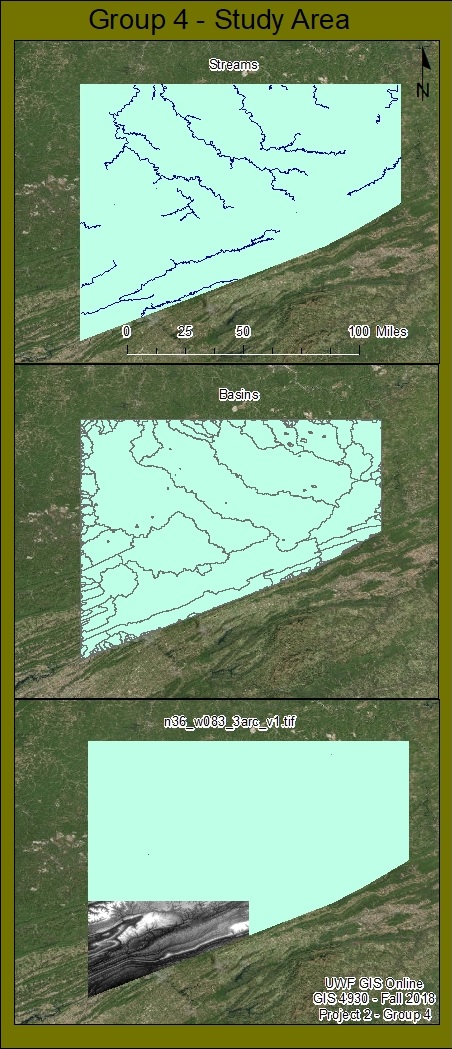
UPDATE: After importing my map files into arcMap and rerunning all tools required to recreate the hydro data files I was successfully able to create the required deliverable for project 2, A single map showing both streams data frame and basins data frame. I've also included a data frame that shows my quadrant (n36_w083_3arc_v1.tif) of group 4's study area for the mountain top removal project.

Link to MTR: 6 stage guide

Link to MTR: Story Map Journal

GIS 4048 - Module 1 Project 1

For module 1 project 1 we were tasked with creating a route map in response to an overturned tractor trailer accident. This proposed incident response message was created in order to distribute to motorists in the area in response to the accident:
"Attention all motorists. An incident involving an overturned tractor trailer has rendered the intersection of Interstates 95 and 945, in Springfield, Virginia, untraversable. As such the following detours have been issued: North to South 3.5 miles, South to East 3.8 miles, South to West 9.8 miles. Please allow for at least a 10 minute delay in your travels today. Thank you."

This map shows detour routes around the incident, proposes routes to designated shelters, informs motorists the extent of the accident, highlights locations of nearby fire stations and all major roadways, shows nearest shelter in color code.

This map was uploaded to arcgisonline.com - 
https://arcg.is/0Kviu9

 

GIS 4035 - Module 3 - LULC classification

For this weeks project, module 3, in GIS 4035 we were tasked with created a land use / land cover classification map for a provided aerial image file. A LULC level II code format was followed and the following codes were applied to the study area and the reasoning for why:

11- Residential - areas that contained buildings that were smaller than commercial size
12 - Commercial and Services - areas that contained larger than home sized buildings and large parking lots
14 - Transportation - main highway
43 - Mixed forest land - all woodland area was categorized under this classification of mixed
51 -  Streams and Canals - smaller streams leading from the bay were categorized as this
53 - Reservoirs - a few small retention ponds in the residential area
54 - Bays and Estuaries - the bay
62 - non-forested wetland - wetland area surrounding the bay that had no trees

GIS 4035 - Module 2 - Visual Interpretation

For my first project in GIS 4035 Photo Interpretation and Remote Sensing, we were tasked with analyzing and interpreting 3 different aerial images.
For the first .tif aerial image file we were tasked with interpreting tone, by classifying 5 polygon feature class files from very light to very dark, and texture, by classifying 5 polygon feature class files from very fine to very coarse.
The following map deliverable was created.

For the next .tif aerial image file we were tasked with interpreting features based on shape, shadow, pattern, and association.  The following map deliverable highlights each of the mentioned features and indicates the color code for that feature in the legend.

For the final .tif aerial image file we were tasked with interpreting color features when compared to a false color IR image of the same study area. The following differences were noted:

Feature	True Color	False Color
Stream	White	Blue
Forest	Green	Red
River	Green-blue	Blue
Building	Light-grey	White
Lot	Dark-grey	Blue